A Tale of Two Coasts
US West Coast became infected by the coronavirus earlier in the epidemic, with the state of Washington having a first officially recorded COVID-19 case on January 19. Many West Coast companies started WFH policies well ahead of the curve, and a few counties in the Bay Area and Seattle issued “shelter in place” orders before the State did. On the other coast, a mayor of the biggest US city urged his fellow citizens to “go on with your lives + get out on the town despite Coronavirus… thru Thurs 3/5 go see “The Traitor” .”
Let’s compare the dynamics of confirmed cases and growth rates between different US states. While many confounding factors, such as population densities, use of public transportation, use of face masks, weather, administrative restrictions, etc. makes it harder to draw clear conclusions, there is a growing consensus that New York situation got substantially worse because of the city’s delayed response.

Data preparation and helper functions
Note: This section is quite technical; if you just want to look at the results of the analysis, you can skip it.
Before we dive into the analysis, let’s gather the data and define a few functions to make the plotting easier. A more detailed description of the data sources and how to use datasets and Entity is provided in two previous posts here and here.
First, let’s combine the information on population and population densities with COVID-19 confirmed cases and deaths. Merge, as it name implies, is used to join two associations by the same key, and the second argument, a pure function that replaces a head of the list with Join, allows us to merge the nested association together, since both of the data structure that we are trying to merge as associations of associations. (If this is unclear, evaluate each of the arguments to Merge separately, inspect and compare it to the result). We also use KeyMap to convert association keys from Entity to String.

Here is the structure of the result:

We do the same for the list of countries; the only difference is that the COVID-19 country dataset splits the data into administrative regions for US, China, Canada, Australia and UK, so we need to combine them to get the total:

Let’s define a function that would normalize timeseries in the following way: first, it will convert the absolute number of cases or deaths into cases per 10K (or 1M) people, to make the numbers between different states and countries comparable. And second, it will truncate all the values below a certain threshold, so that when we compare the growth over time, all the curves start (roughly) in the same place.

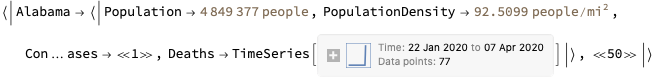
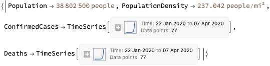
For example, here is the entry for California:

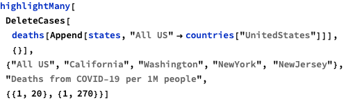
and here is the deaths per million since the day they exceeded 1:


We will also create shortcuts for cases and deaths that can be applied to whole associations:

Finally, let’s define some plotting routines. Since 50 US states (or 251 countries) is much to display on the same graph, we’ll define a function to plot selected lines with colors and labels, while plotting everything else with thin gray lines to create a context.


A Tale of Two Coasts
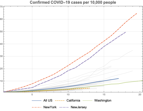
As we mentioned in the beginning, West Coast states were more proactive than East Coast states in implementing WFH and quarantine measures. Add lower population density and significantly smaller public transportation, and you will see a drastically different picture in terms of both number of confirmed cases:

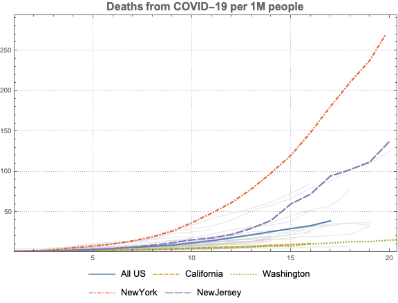
and number of deaths:
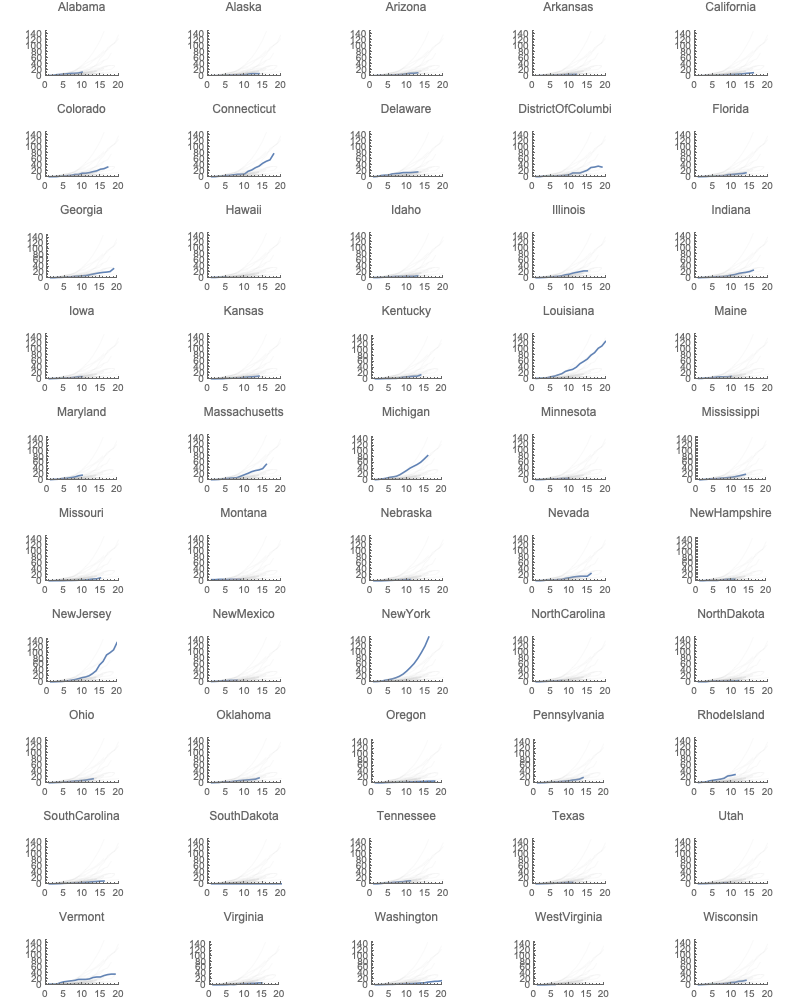
Here is a full grid showing data for each individual state, for both confirmed cases:

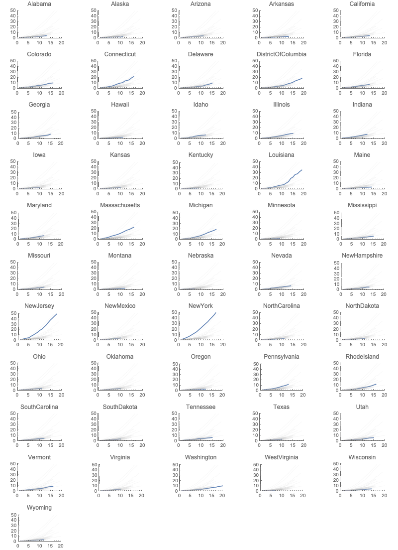
and deaths for those cases that have more than 1 per 1M:

Population density and other factors
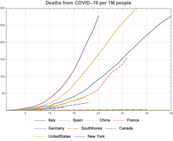
To put New York numbers in the perspective, let’s compare them to aggregates for a few countries. Let’s see how it compares to Italy and Spain that didn’t do so well, as well as to South Korea - a place with a high population density, as Seoul’s population is 10M people is over 20% of the country’s total.
As you can see, New York substantially dominate all of these countries. South Korea is barely visible at the bottom of the chart, as they have managed the pandemic exceptionally well, with ~4 deaths per 1M. In other observations, overall US numbers track France surprisingly well, and situation is much worse in Spain now that in Italy, which was the original “hot bed” in Europe, with France almost caught to Italy.